Working with open-ended survey responses(1): examine texts

Researchers have mixed feelings towards the use of open-ended questions and their dislikes partially come from the difficulty of post-processing text data that they collected from the questions. In this post and the next, I’ll illustrate how to examine and deal with short text answers in Python.
If you think about what open-ended questions usually ask, it could be unaided recalls (e.g. what’s in you mind when you think of XX), asking the whys (e.g. you mentioned you XX, can you tell me why?), or short answers responding to other-please specify. There are various types of open-ended questions, and it’s better to choose the right tool to deal with them for efficiency.
I will keep using the same survey dataset that I have been using for my previous posts in this series, feel free to check them out here: post1, post2, post3.

import numpy as np
import pandas as pd
from wordcloud import WordCloud
import matplotlib.pyplot as plt

df = pd.read_parquet('../output/df')

In this dataset, it’s interesting to see that gender is not collected by a multiple question that we are familiar with. Instead of asking respondents to choose from a list of standard options such as Male, Female, this study used an open-ended text field that collected respondents’ text descriptions of their gender.

Examine short text answers

len(df['gender'].unique())

71

df['gender'].value_counts().head(5) # display the top 5

Male      610
male      249
Female    153
female     95
M          86
Name: gender, dtype: int64

df['gender'].value_counts().tail(5) # display the bottom 5

Genderfluid (born female)       1
Male (trans, FtM)               1
Other/Transfeminine             1
Bigender                        1
Female or Multi-Gender Femme    1
Name: gender, dtype: int64

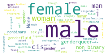
So looks like there were 71 kinds of responses, including variations of gender descriptions and spelling/lower/upper casing kind of variations. I’ll first transform all text into lowercase and create a wordcloud to quickly visualize it.
Note it’s worth considering whether making all texts into lowercase/uppercase is a good choice for your text since some nuances could be captured by the capitalization of letters. In my case here, I wouldn’t mind changing all texts to lower case.

df['gender'] = df['gender'].str.lower()

gender_list = df['gender'].to_list()
text = " ".join(str(x) for x in gender_list)

wordcloud = WordCloud(background_color='white').generate(text)
plt.imshow(wordcloud, interpolation='bilinear')
plt.axis("off")
plt.show()

With wordcloud and matplotlib libraries, we could create a simple wordcloud (without any customizations) just to have a feeling of what answers were generally included in the responses.

Here we could design a numbered value scheme and quickly code male and female into 1 and 2 respectively. We could researve 0 for non-binary.

df['gender_r'] = 0
df.loc[df['gender'] == 'male', ['gender_r']] = 1
df.loc[df['gender'] == 'female', ['gender_r']] = 2

df['gender_r'].value_counts().sort_index()

0    325
1    860
2    248
Name: gender_r, dtype: int64

Looks like we have 325 text answers that need to be further checked. I’m interested in what these answers look like and I would print out the top 5 most frequent descriptions of gender:

df.loc[df['gender_r']==0, ['gender']]['gender'].value_counts()[0:5]

m              165
f               61
woman            7
man              5
non-binary       4
Name: gender, dtype: int64

df.loc[df['gender'] == 'm', ['gender_r']] = 1
df.loc[df['gender'] == 'f', ['gender_r']] = 2
df.loc[df['gender'] == 'woman', ['gender_r']] = 1
df.loc[df['gender'] == 'man', ['gender_r']] = 2

df.loc[df['gender_r']==0, ['gender']]['gender'].value_counts()[0:10]

non-binary              4
cis male                3
nonbinary               2
genderqueer             2
human                   2
agender                 2
male (cis)              2
genderflux demi-girl    1
fluid                   1
fm                      1
Name: gender, dtype: int64

Frequency output shows that the texts haven’t been fully cleaned yet. For example, “cis male” and “male (cis)” could be categorized into male.

Search for substring

We could run a simple search for substring to determine whether it should be categorized to either gender category or not.

# exclude cleaned text answers
uncleaned_textdf = df.loc[df['gender_r']==0, ['ID', 'gender']]

The use of in is pretty simple - after search substring within string it will return a boolean value (True or False). See an example below:

'male' in 'male (cis)'

True

# create a simple function that process data in batch
def checksubstring(substring, listofstring):
    booleanlist=[]
    for text in listofstring:
        booleanlist.append(substring in text)
    boolean_dic = {'text': listofstring,
                   'check': booleanlist}
    boolean_df = pd.DataFrame(boolean_dic)
    return boolean_df

checksubstring('female', uncleaned_textdf['gender'].dropna())[0:5]

	text	check
16	i identify as female.	True
29	bigender	False
30	non-binary	False
42	female assigned at birth	True
103	fm	False

You probably noticed that this isn’t the best tool to use as simply by searching “male” and assigning it back to the “male” category, we may mis-catgorize those that for example mentioned “male/genderqueer”. For only around 60 uncategorized texts, it’s probably easier to just manually review and code them to the appropriate categories. Sometimes, we/human could work with computer to acheive the best performance and highest efficiency.

Another way to deal with texts is to use word embeddings from the very beginning. I’ll illustrate this method a bit more in the upcoming posts.